Chapter 1 Learning spoken words with multiple possible spellings
Work presented in this chapter is based on:
1.1 Introduction
The first experimental chapter of this thesis further explores the orthographic skeleton hypothesis by testing whether orthographic skeletons are generated for all novel words acquired via aural instruction, or only for words with a unique, and hence completely predictable spellings. Understanding the conditions under which orthographic skeletons are generated - or not - will shed light on how lenient the mechanism that drives phoneme-to-grapheme conversions is, and specifically, show whether it is constrained by spelling uncertainty. The idea, along with the supporting experimental evidence, that orthographic representations can be generated solely based on novel word’s phonological form, have already been described in the introduction. Here, we will focus on questions that remained open, and which consequently motivated the present study.
Firstly, we saw that Wegener and colleagues (2018) manipulated the predictability of novel spoken words’ spellings and showed a significant reading facilitation only for previously trained words with predictable spellings. The absence of facilitation for trained words with unpredictable spelling was interpreted as stemming from a mismatch between the correct spelling (i.e., the one children were presented with) and the one they generated during aural training (i.e., the orthographic skeleton generated during the learning phase). The authors thus concluded that orthographic representations for novel words can be generated solely based on the phonological properties of novel words, and importantly, that this occurs prior to readers’ first visual encounter with words’ actual spellings. Nevertheless, although their data provide strong evidence for the orthographic skeleton hypothesis, it remains unclear if the absence of the processing facilitation observed for words with unpredictable spellings, was caused by a mismatch between inaccurate orthographic representations children generated and the spellings they were presented with, as argued by the authors, or rather because children did not generate any representations for these words at all. Namely, it could have been the case that children did not even engage in the process of generating orthographic expectations when uncertainty regarding potential spellings was high. The first and the main goal of the present study was thus to test whether orthographic skeletons are generated even when there is uncertainty regarding the correct spelling (i.e., for words with more than one possible spelling), or only when words have a unique possible spelling. A way to adjudicate between these two possibilities, would be to train participants on a set of novel words controlled for the number of possible spellings. The idea being that, if a word has only one possible spelling, all participants would generate the same orthographic representation. If a word has multiple potential orthographic representations however, it is difficult to predict, on a participant level, whether orthographic representations would be generated, and if so, which of the possible and legal spelling option would be used to generate such representation. This leads us to the second goal of the present study. Namely, Johnston et al. (2004) pointed out that the spellings participants were presented with in their task might not have coincided with those they had previously generated. In particular, spelling expectations participants generated could have been different from those the experimenters provided in the task. However, if participants generate orthographic expectations even when multiple options are possible (i.e., under uncertainty), they should generate a one specific representation (selected from the possible options). This preferred spelling option, and the one likely to be used to generate the orthographic skeleton, could in some cases be based on statistical properties of languages (Davis & Perea, 2005). Nevertheless, as different spelling options can sometimes be equally possible (the case of the sound /b/ in Spanish; see below), it is difficult to predict which one would be used to generate a novel orthographic representation. Generating orthographic skeletons could thus, at least partly, be influenced by individual preferences. Therefore, as a second goal we wanted to see whether - if indeed generated - orthographic skeletons for words with more than one spelling follow individual spelling preferences.
Both of the aforementioned studies were conducted in English, an opaque language with extremely complex phoneme-to-grapheme conversion rules. Due to both irregular spellings and complex phoneme-to-grapheme mappings (English has 44 phonemes that can map onto more than 200 different graphemes), creating novel words with either a unique or only two possible spellings would be challenging, if not impossible. As a result, both predictable and unpredictable items are likely to have more than one possible spelling. Therefore, to control for the number of possible spellings and test whether orthographic skeletons are generated even under uncertainty, speakers of a more transparent language which allows us to better control for the number of possible spellings should be tested.
Contrary to English, Spanish orthography is made up of relatively simple phoneme-to-grapheme conversion rules (a total of 24 phonemes that map onto 32 graphemes). Crucially for the goal of the present study, most of the phonemes map onto only one grapheme (e.g., phonemes /m/ and /t/ can only be written as <m> and <t> respectively), and almost all vowels are completely consistent. This implies that there are many words (and consequently, pseudowords) whose spellings can be entirely predicted from their phonology, given that they have only one possible orthographic representation (e.g., the pseudoword /dalu/ can only be written as <dalu> in Spanish). At the same time, Spanish contains few inconsistent phonemes which have two orthographic representations (i.e., graphemes). The example that best illustrates Spanish orthographic inconsistency is the case of the sound /b/, which in Spanish maps either onto the letter <b>, or the letter <v>. Consequently, if only one sound in a particular word is inconsistent, that word would have exactly two (and not more) legal spellings (e.g., /bupe/ can be spelled as <bupe> or <vupe>). This property of the Spanish language provides a methodologically accurate way of controlling the predictability of novel word spellings: creating words with either only one or only two possible spellings. As as result, this enable testing whether orthographic skeletons are generated regardless of any uncertainty related to phoneme-to-grapheme mappings (both for words with a unique as well as those with those legal spellings) or are generated only when there is no uncertainty (i.e., only for words with a unique spelling such as /dalu/).
1.1.1 The present study
Experiment 1 aimed to further explore the orthographic skeleton hypothesis by testing whether orthographic representations are generated for all newly acquired spoken words or only for words with a unique and hence completely predictable spelling. To this end, a group of Spanish-speaking adults was trained on pronunciations of novel words with either only one (hereafter consistent words) or two possible spellings (hereafter inconsistent words). Namely, consistent words were made of phonemes with a unique possible grapheme representation in Spanish. As a result, spellings of these words were completely predictable from their phonology (e.g., /sufe/ can only be written as <sufe> in Spanish). By contrast, initial phoneme of all inconsistent words had two grapheme representations giving this way words two possible spellings (e.g., /χepo/ can be spelled either as <gepo> and <jepo>). Given that word spelling depends strongly on the graphotactic rules of a language (Carrillo & Alegría, 2014), for some words, the preferred spelling could be inferred and predicted based on bigram frequencies, as one of the two possible grapheme representations may be more likely to appear in a specific context. For instance, the phoneme /χ/ is more likely to be represented with the grapheme <g> when followed by the vowel /i/. For some Spanish phonemes however, it is more difficult to predict which grapheme is more probable to appear in a certain context given that the two representations have balanced frequencies (e.g., the sound /b/ followed by vowels /a/ or /o/ can be represented with either <b> or <v>, with similar frequencies in the language). This makes it difficult to anticipate, at the group level, which spelling would be preferred between the two options and consequently which would be used to generate an orthographic skeleton, if it is indeed generated despite uncertainty. Thus, there was a need to access participants’ preferences for any of the two possible spellings. To account for possible individual differences in spelling preferences, we obtained obtained them beforehand. Namely, two weeks before the aural training took part, all participants provided their spelling preferences for all novel words (as well as some filler words; see Section 1.2.3.1). These preferences were used to present half of inconsistent words in each participant’s preferred spellings and the other half in their unpreferred spellings. We assumed that if participants generate orthographic skeletons for aurally acquired words with two spellings, these orthographic skeletons would be based on individual preferences (i.e., the spelling option participants had provided beforehand).
Predictions regarding the outcomes of the study were the following. On the one hand, if participants generate orthographic expectations even when a word has more than one possible spelling, similar reading times should be observed for consistent and inconsistent words shown in their preferred (i.e., likely to be predicted) spelling. By contrast, words shown in their unpreferred spellings should elicit longer reading times indicating a mismatch between the expected and the real spelling. Given that this pattern should only be observed in the set of words participants had previously been trained on (i.e., trained words), a significant interaction between training and spelling should be found. As in Wegener et al. (2018), this interaction should be driven by a facilitation present when reading trained as compared to untrained words. Alternatively, the interaction could stem from significantly longer reading times present only for inconsistent unpreferred trained words (yielding a surprisal effect). On the other hand, if participants generate orthographic expectations only for words with one possible spelling, reading times should be faster for consistent (e.g., /dalu/) than for inconsistent (e.g., /χepo/) trained items regardless of the spelling (i.e., consistent words should be read faster as compared to either preferred or unpreferred inconsistent words). An interaction between spelling and training could be driven either by a facilitation present only for consistent trained words or by longer reading times observed for all inconsistent trained words (both preferred and unpreferred). Finally, no differences between the three spellings should be observed in the set of untrained words, given that in this case, no orthographic expectations could have been generated prior to the first visual encounter.
1.2 Methods
1.2.1 Participants
In order to have the equal number of participants across all experimental lists (see Section 1.2.3.3) as well as have a similar number of participants as were tested by Wegener et al. (2018), a sample size of 48 participants with usable data was determined before data collection.
A total of 54 participants completed the first session of the experiment. Due to technical issues three of them were not able to complete the second session and additional three participants had to be excluded from the analysis due to low accuracy in the aural training task. Data reported here come from the 48 participants (44 female) aged between 18 and 35 years (M = 25.6, SD = 3.74) who completed both experimental sessions within 14 to 16 days. All participants had Spanish as their first and dominant language, and their language skills were assessed through a series of objective proficiency measures: an interview conducted by a native Spanish speaker rated from 1 (lowest level) to 5 (native or native-like level), a picture naming task (the BEST proficiency test; de Bruin, Carreiras, & Duñabeitia, 2017), a lexical decision task (i.e., LexTALE-Esp which is the Spanish version of the LexTALE language proficiency test; Izura, Cuetos, & Brysbaert, 2014). In addition, subjective measures of proficiency were obtained through participants’ self-reports on different aspects of proficiency. Namely, writing, listening, understanding, and speaking (see Table 1.1 for complete information about participants language profile). Participants were recruited from the BCBL Participa database and each received 15 euros for their participation in the study. The experiment was entirely web-based, but all participants had previous experience in participating in behavioral experiments in the laboratory and were therefore familiar with procedures and tasks used in experimental psychology (Uittenhove, Jeanneret, & Vergauwe, 2022). The experiment was approved by the BCBL Ethics Review Board (approval number 060420MK) and complied with the guidelines of the Helsinki Declaration. Participants’ written consent was collected at the beginning of each experimental session.
| Mean | SD | Range | |
|---|---|---|---|
| AoA | 0 | 0 | 0-0 |
| Picture naming (0-65) | 64.7 | 0.54 | 63-65 |
| LexTale (0-100%) | 93 | 6.24 | 71.7-100 |
| Interview (1-5) | 5 | 0 | 5-5 |
| Self-rated proficiency (0-10) | |||
| Speaking | 9.65 | 0.64 | 7-10 |
| Understanding | 9.64 | 0.61 | 8-10 |
| Writing | 9.45 | 0.77 | 7-10 |
| Reading | 9.51 | 0.75 | 7-10 |
| Note. Some participants had some knowledge of a second or even a third language but none was highly proficient in any language other than Spanish. | |||
| a There are a total of 65 pictures to be named in the BEST (making 65 the maximum possible score). b Self-rated proficiency data are missing for one participant. |
1.2.2 Stimuli
1.2.2.1 Novel words
Two sets of four-phoneme-long disyllabic novel words with the CVCV structure were created (set A and B, used as Trained and Untrained items and counterbalanced across participants). Each set consisted of eight consistent and 16 inconsistent words. Consistent words contained phonemes that map onto only one grapheme in Spanish. Consequently, consistent words had a unique possible spelling (e.g., /dalu/ can only be written as <dalu>). Inconsistent words by contrast, always stared with phonemes that had two possible orthographic representations in Spanish: /b/ which can be written as <b> or <v>; /k/ which when followed by vowels /i/ or /e/ can be written as <qu> or <k>; /ʎ/ which maps onto <ll> or <y>, and /χ/ which before vowels /i/ and /e/ has two orthographic representations <j> or <g>. This way, all inconsistent words had two legal spellings in Spanish (e.g., pseudoword /ʎedu/ can be written either as <lledu> or <yedu>). Half of the inconsistent words were a priori labeled as preferred and half as unpreferred. Preferred and unpreferred spellings were obtained for each participant individually through a pseudoword spelling task (see Section 1.2.3.1). Both preferred and unpreferred items contained two words starting with each of the four target inconsistent phonemes. Across preferred and unpreferred inconsistent items, words were also matched on the first syllable (two syllables per phoneme). Therefore, both preferred and unpreferred items started with the following eight syllables: /ʎe/ and /ʎu/, /χe/ and /χi/, /ba/ and /bu/, /ki/ and /ke/ (see Table 1.2).
| Set | Consistent | Inconsistent Preferred | Inconsistent Unpreferred |
|---|---|---|---|
| A | |||
| A | /dalu/ | /ʎedu/ | /ʎefo/ |
| A | /duti/ | /ʎuɲe/ | /ʎupo/ |
| A | /femi/ | /χepo/ | /χede/ |
| A | /fipu/ | /χifo/ | /χitu/ |
| A | /ludi/ | /bamu/ | /badi/ |
| A | /nepo/ | /bupe/ | /bumi/ |
| A | /panu/ | /kime/ | /kifo/ |
| A | /muni/ | /ketu/ | /keli/ |
| B | |||
| B | /dopu/ | /ʎepo/ | /ʎeli/ |
| B | /fadi/ | /ʎule/ | /ʎufi/ |
| B | /leme/ | /χeni/ | /χetu/ |
| B | /mepu/ | /χipe/ | /χidu/ |
| B | /nute/ | /bafu/ | /bani/ |
| B | /pimu/ | /buɲe/ | /buti/ |
| B | /sufe/ | /kipe/ | /kiɲo/ |
| B | /tamu/ | /kefi/ | /kedi/ |
| Note. Words from the inconsistent preferred group were later shown in each participant’s preferred spelling whereas words from the inconsistent unpreferred group were presented in the unpreferred spelling. | |||
Consistent items were matched between the two sets on the number of orthographic neighbours (no word had more than three neighbours, Set A: M = .750, SD = 1.04 and Set B: M = 1.38, SD = 1.22, t(14) = -1.12, p = .281) and neither of the two possible spellings of inconsistent words had more than three orthographic neighbours. In order to avoid a potential gender mismatch between the demonstrative pronoun <este> preceding the novel in all experimental sentences (see Section 1.2.3.3) none of the novel words ended with the vowel /a/, as it most often marks the feminine gender of the nouns in Spanish (although there are some exceptions, e.g., \(mano_{feminine}\)). All items were recorded by a male L1 speaker of Spanish coming from the same region of Spain as the participants tested in the study. The recordings were made in a sound attenuated cabin using Marantz PMD661.
1.2.2.2 Novel objects
A total of 48 pictures selected from The Novel Object and Unusual Name (NOUN) Database (Horst & Hout, 2016) were used as the novel objects participants were presented with in the experiment (see Figure 1.1). Pictures were selected so as to be as different as possible from each other and were then randomly associated with novel words (see Table 1.2). Novel words and pictures associations were then kept constant for all participants (i.e., the same object was associated with the same word for all participants).
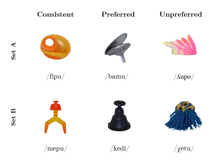
Figure 1.1: Novel Objects from Experiment 1. An example object from each set (set A and set B) and spelling group (Consistent, Preferred, and Unpreferred).
1.2.3 Procedure
The experiment was divided into two sessions, both completed online using the OSWeb online runtime, a JavaScript implementation of OpenSesame 3.3.2 software (Mathôt, Schreij, & Theeuwes, 2012) and hosted on the JATOS testing server (Lange, Kühn, & Filevich, 2015). All participants completed two experimental sessions with a two week pause in between them. Both sessions started with the audio message instructing participants to use headphones throughout the entire experiment as well as to make sure the sound is adjusted to a comfortable level.
During Session 1 participants first completed a pre-test spelling task, which aimed at assessing their individual spelling preferences. To mask the preferred spelling manipulation, during the same session participants completed two filler linguistic tasks: a lexical decision task followed by a real word spelling task. Tasks were always presented in this order so as to avoid any orthographic influence from the distractor tasks on the pre-test spelling task. Since these tasks were not of interest for the study, they will no be further discussed.
Session 2 always started with the aural training task during which participants were trained on the names of 24 novel objects. Next, they did a short distractor task (i.e., the Simon task; Simon, 1969) which was immediately followed by a self-paced reading task. In the self-paced reading task participants were for the first time exposed to the written forms of words they had previously been trained on. After the reading task, participants completed a short picture naming task in which they saw the pictures of all the objects they had been trained on and were instructed to name/spell them by typing the name of each object as they appeared one by one on the screen.
Finally, at the end of experiment participants were asked to answer several questions regarding the possible strategies they employed while doing the experiment, as well as hear their impressions about the tasks. They were also explicitly asked to indicate whether the spellings they were presented with differed from the ones they expected to see.
1.2.3.1 Pre-test spelling task
The aim of the pre-test spelling task was to obtain participants’ individual spelling preferences and determine the preferred and unpreferred spellings of inconsistent words for Session 2. These preferences were then used to present words from the preferred group in spellings participants provided (i.e., preferred spellings), and those from the unpreferred group in the other, non-preferred spellings. For instance, if a participant spelled /bamu/, which belongs to the preferred group (see Table 1.2), with <b> in Session 1, that same participant would then see this word written with <b> in Session 2. By contrast, if a participant wrote /badi/, which belongs to the unpreferred group (see Table 1.2, with <b> in Session 1, that same participant would see the word written with <v> in Session 2.
Participants were presented with a total of 96 novel words, half of them target (see Table 1.2) and half filler (see Table ??). Filler words were created using the same phonemes and first syllables as the target words, and were added to ensure that participants would not remember, two weeks later during the aural training task, that they had already heard these novel words during Session 1. Participants were instructed to spell the novel words as if they were real words in Spanish (i.e., following the orthotactic rules of Spanish).
Novel words were presented in a randomized order and the task was self-paced. On each trial participants first heard a novel word over headphones and were prompted to spell what they heard in the text box appearing below the question “Please spell the word you just heard”. After typing in their response, they had to press ‘enter’ to move on to the next trial and hear the next novel word. The task took participants around 10 minutes to complete.
1.2.3.2 Aural training
During the aural training task, participants were trained on the names of 24 novel objects taken from one the two sets (set A or set B which were counterbalanced across participants). They were instructed to learn the names of all objects since their performance would be tested later on in the experiment. In order to internalize the masculine gender of the nouns during the training phase, and thus avoid possible gender mismatch in the self-paced reading task (see Section 1.2.3.3), participants were explicitly told that the names of all objects were masculine.
With the aim to limit the learning load, novel objects and their corresponding names were presented in four blocks of six. Each block was made up of two words belonging to each of the three spelling groups (i.e., two consistent, two preferred and two unpreferred) and was split into two parts: exposure and practice part (see Figure 1.2). In the exposure part, participants were presented with the pictures of six novel objects. Pictures were presented one by one at the centre of the screen and at the same time the picture was presented, its name was played three times in a row at different speeds. The first and the third time, the name of the object was pronounced entirely, whereas the second time, it was pronounced by separating and emphasizing each of the two syllables (e.g., /muni/ -> /mu/ - /ni/ -> /muni/). After hearing the name of the object three times in a row, participants could press ‘enter’ in order to proceed to the next trial. Once they had been exposed to all six objects, they initiated the practice part. In the practice part, two different objects appeared on the left and on the right side of the screen, and at the same time, the name of one of them was played. Participants had to select the picture that corresponded to the name they heard by pressing ‘M’ or ‘Z’ on the keyboard (for picture on the right versus on the left). To reinforce the training process each trial was immediately followed by a feedback message (happy or sad face). Each picture was paired with every other picture and appeared once on the left and once on the right side of the screen, giving this way a total 60 trials in each practice block. At the end of each block, participants received a feedback message informing them about their overall accuracy rate (in %) in that practice block. This same procedure was repeated for all four blocks of words, and participants were encouraged to take breaks after each block.
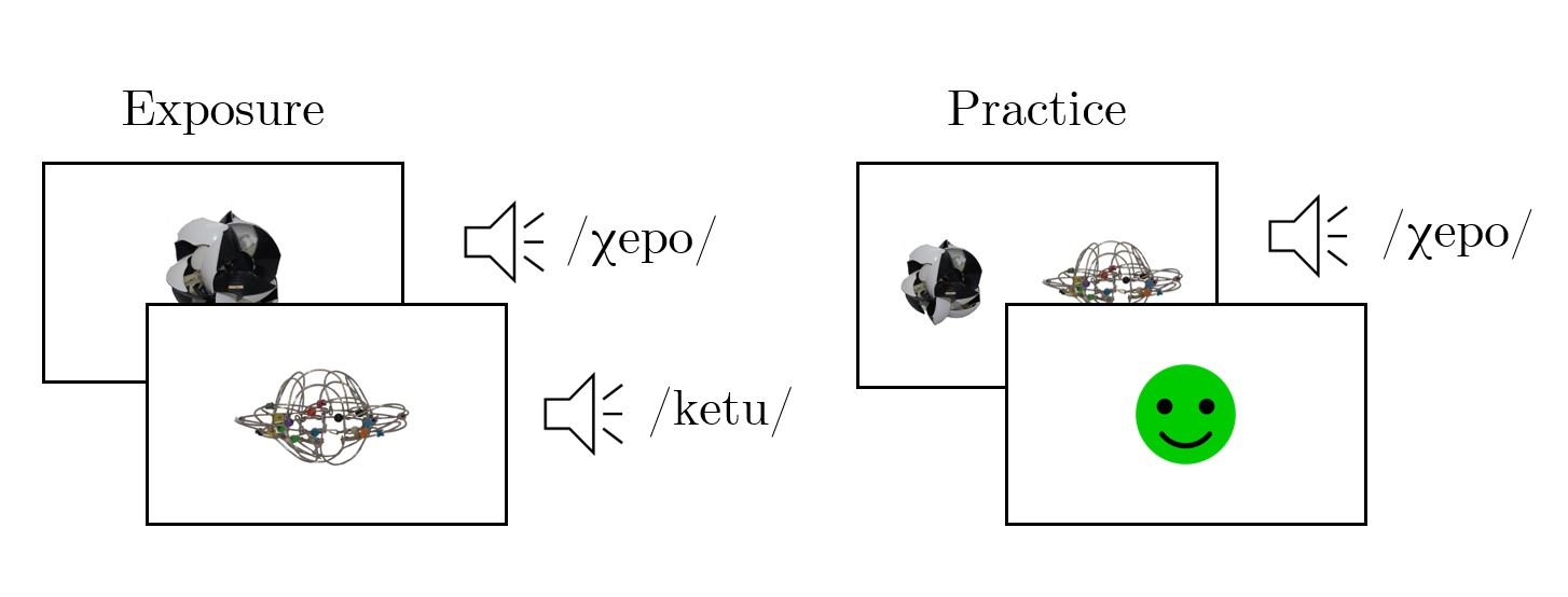
Figure 1.2: Trials of the Aural Training Blocks. In the exposure part (left), participants were presented with each of the six objects from that block one by one, while listening to their names spoken three times in a row. In the practice part, they saw two objects on the screen and heard the name of one of them. Participants had to select the object that corresponded to the name they had heard by pressing either ‘M’ (right) or ‘Z’ (left) on their keyboard.
Once all 24 objects had been presented and participants were trained to recognize their names, they completed the final block of the aural training task. In this block, participants were first presented with all 24 objects once again. Objects were presented one by one at the centre of the screen and at the same time, their names were played through headphones. As in the previous blocks, the exposure was self-paced, and participants moved from one picture to the next one by pressing ‘enter’ on their keyboard. After being familiarised once again with the names of all objects, they completed the final practice task. This time, four objects were presented on the screen, two on the left and the right side of the screen, and two on the upper and lower part of the screen (see Figure 1.3). As in the previous practice phases, at the same time the pictures were presented on the screen, participants heard the name of only one of them. To respond to which object on the screen corresponds the name they had heard, they had to use one of the four arrows on the keyboard (see Figure 1.3). To make sure that each picture appeared the same number of times at each of the four positions on the screen, and was paired equally with every other picture, position and pairing of the pictures was counterbalanced through Latin square, giving a total of 144 trials. As in the previous practice phases, participants received feedback message indicating whether their response was correct immediately after each trial. They also received the final feedback message informing them about their overall performance at the end of the task. On average participants needed approximately 30 minutes to complete the aural training task.
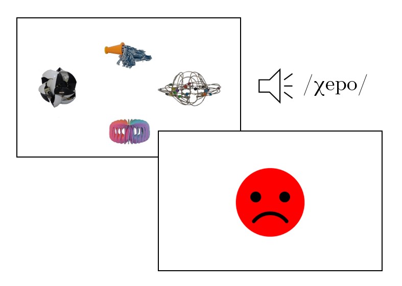
Figure 1.3: Final Block of the Aural Training Task. On each trial participants were presented with four objects on the screen and at the same time they heard the name of only one. After giving their response participants received a feedback message indicating whether the response was correct.
1.2.3.3 Self-paced reading task
In the self-paced sentence reading task participants were presented with consistent, preferred and unpreferred spellings of the 24 words they had been trained on (i.e., trained words), as well as the 24 words from the other set (i.e., untrained words). Spellings of the words were embedded in eight different four-to-seven words long sentences (see Table 1.3). To make sure each target word appears the equal number of times in each sentence structure, and each of the six possible positions in the sentence (from two to seven), the position of the target word in a sentence was counterbalanced across the participants using the Latin square procedure. This yielded eight different sentence combinations repeated three times for the trained and three times for the untrained words (each participant read 48 sentences in total). Note that varying the length of the sentences, as well as the position of the target word within the sentence, was made to avoid the anticipation of the target word during reading (i.e., the moment of target word display within each sentence was unpredictable). Apart from making the task more engaging, the unpredictable position of the target word ensured that participants actually read the words, and do not just press ‘enter’ without processing them.
| Original sentence | English translation |
|---|---|
| Este xxx es pequeño | This xxx is small |
| Este gran xxx es bonito | This big xxx is pretty |
| Este es un xxx grande | This is a large xxx |
| Este es un pequeño xxx fantástico | This is a small fantastic xxx |
| Este objeto es un xxx pequeño | This object is a small xxx |
| Este objeto es un pequeño xxx bonito | This object is one small fantastic xxx |
| Este gran objeto es un xxx fantástico | This big object is one fantastic xxx |
| Este gran objeto es un fantástico xxx | This large object is a fantastic xxx |
| Note. Due to syntactic differences across languages the position of the target word is not equivalent in the Spanish sentences and their English translations . Exes represent the place where target words appeared. |
Sentences did not provide a rich semantic context but were preceded by a picture of the object whose named appeared in the sentence, this way priming the target word. Sentences were presented in a randomised order and the exact structure of each trial was the following: first a fixation cross appeared at the centre of the screen. After 500ms it was replaced by the picture of the object which stayed on the screen for a total of 2000ms. The picture was then replaced by a blank screen and after 1000ms the first word of the sentence appeared. The first word was the same across all sentences (i.e., each sentence started with the same demonstrative pronoun <Este>). From this point on, the task was self-paced and participants moved from one word to the next one by pressing ‘enter’ on their keyboard. After reading the last word of the sentence, participants initiated the beginning of the next trial by pressing ‘enter’ on their keyboard (See Figure 1.4). Participants were instructed to read each sentence as fast as possible without making pauses on any particular word. They were provided with six practice trials during which three sentences preceded by three familiar objects (e.g., a book, a glass and a pencil) were presented two times. Participants’ reaction times, measured relative to the onset of the target word at the centre of the screen, were recorded and used as the index of their reading times. The entire task took participants around 10 minutes to complete.
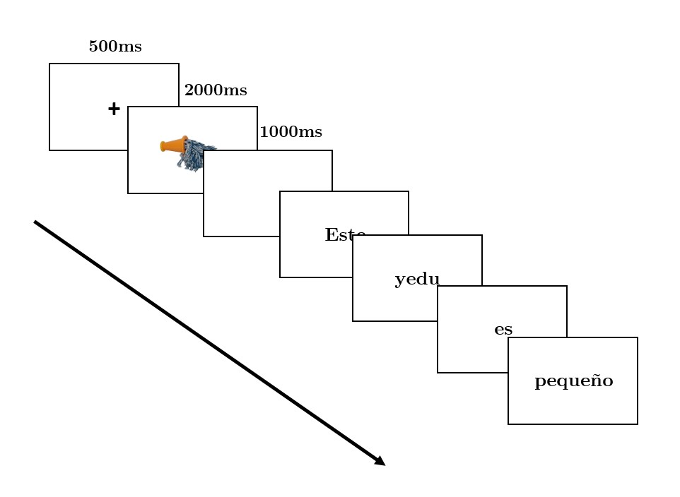
Figure 1.4: The Structure of the Trial in the Self-Paced Reading Task. Each trial started with a fixation cross present for 500ms at the centre of the screen. The fixation cross was replaced by the picture of the object whose name was to appear in the following sentence. After 2000ms the picture of the object was replaced with a blank screen. The first word of the sentence appeared after 1000ms. Words appeared one-by-one at the center of the screen and the task was self-paced.
1.2.3.4 Picture Naming Task
At the end of the experiment participants were presented with the pictures of the 24 objects they had been trained on, and were instructed to name them by spelling/typing their names. Pictures were presented in a randomised order one by one at the centre of the screen with the following trial structure: first, the picture of an object appeared at the centre of the screen. After 1000ms the picture became smaller, and a text box appeared below it, prompting participants to type in the name of the object shown on the picture. After writing the name of the object participants moved on to the next trial by pressing ‘enter’ on their keyboard. The aim of this task was to see how well participants could recall the names of the words they were trained on. The duration of the task was approximately five minutes to complete.
1.2.4 Data pre-processing and analysis
Data from the pre-test spelling task are presented in Appendix 3.6 (see Table ?? and ??). Since they were only used to obtain individual spelling preferences, these data will not be further discussed.
To be included in the analysis of reading times (see Section 1.2.4.1) participants had to obtain at least 70% of accuracy in the aural training task. As data from the aural training task served only as an indicator of whether participants acquired the phonological forms of novel words they had been trained on, only descriptive statistics for the phonological training will be shown.
1.2.4.1 Self-paced reading task
Reaction times for both trained and untrained words from the self-paced reading task were analyzed using linear mixed effects models (R. H. Baayen, Davidson, & Bates, 2008) in the statistical environment R (Version 4.2.0; R Core Team, 2021) and the R-packages }dplyr [@}R-dplyr], designr (Version 0.1.12; Rabe, Kliegl, & Schad, 2021), forcats (Version 0.5.1; Wickham, 2021), ggplot2 (Version 3.3.6; Wickham, 2016), huxtable (Version 5.5.0; Hugh-Jones, 2022), hypr (Rabe, Vasishth, Hohenstein, Kliegl, & Schad, 2020; Version 0.2.2; Daniel J. Schad, Vasishth, Hohenstein, & Kliegl, 2019), kableExtra (Version 1.3.4; Zhu, 2021), knitr (Version 1.39; Xie, 2015), lme4 (Version 1.1.29; Bates, Mächler, Bolker, & Walker, 2015), lmertest (Kuznetsova, Brockhoff, & Christensen, 2017), MASS (Version 7.3.56; Venables & Ripley, 2002), papaja (Version 0.1.0.9999; Aust & Barth, 2022), purrr (Version 0.3.4; Henry & Wickham, 2020), readr (Version 2.1.2; Wickham, Hester, & Bryan, 2022), readxl (Version 1.4.0; Wickham & Bryan, 2022), stringr (Version 1.4.0; Wickham, 2019), tibble (Version 3.1.7; Müller & Wickham, 2022), tidyr (Version 1.2.0; Wickham & Girlich, 2022), tidyverse (Version 1.3.1; Wickham et al., 2019), tinylabels (Version 0.2.3; Barth, 2022), and xtable (Dahl, Scott, Roosen, Magnusson, & Swinton, 2019; Version 1.8.4; Hugh-Jones, 2022) were used for data analysis and visualisation.
Before analyzing reaction times (RTs), extreme values (i.e., RTs below 150ms and above 1200ms, representing 4.9% of the data) identified based on the visual inspection of the raw data were removed (Ratcliff, 1993; see also R. H. Baayen & Milin, 2010). 4 In line with the Box-Cox test (Box & Cox, 1964) RTs were then log transformed in order to improve the positively skewed distribution, as well as minimize the effects of any possible outliers (R. Baayen, 2008).
To test whether there was a significant difference in reading words with a unique spelling (i.e., consistent words) and each of the two inconsistent spellings (i.e., inconsistent preferred and inconsistent unpreferred spellings), the three level factor group spelling was deviation coded (Daniel J. Schad, Vasishth, Hohenstein, & Kliegl, 2020). The first contrast thus compared the RTs between consistent and inconsistent preferred spellings (hereafter Spelling1vs2; consistent spellings were coded as -0.33, inconsistent preferred as 0.67 and inconsistent unpreferred as -0.33) while the second contrast compared consistent to inconsistent unpreferred spellings (hereafter Spelling1vs3; consistent spellings were coded as -0.33, inconsistent preferred as -0.33 and inconsistent unpreferred as 0.67). The fixed factor Training was initially deviation coded (trained words were coded as 0.5 and untrained as -0.5). In case of a significant interaction between training and either of the two contrasts, training was treatment coded (i.e., the level of interest was coded as 0 and the other as 1) in order to change intercept and thus look at the simple effects of the contrast either at the level of trained words only (trained as 0 untrained as 1) or untrained words only (trained as 1 untrained as 0). In addition, the two-level factor Set representing to two sets of items, was deviation coded (Set A as -0.5 and Set B as 0.5) and included in the model as the fixed covariate.
To avoid overfitting the statistical models which would lead to reduced statistical power (Matuschek, Kliegl, Vasishth, Baayen, & Bates, 2017), random-effects structure was build following a parsimonious data-driven approach (Bates, Kliegl, Vasishth, & Baayen, 2015). As a result, all reported models represent the highest nonsingular converging models and include the maximal random effects structure for all experimental manipulations of interest supported by the data (see Table 1.5 for exact model structure).
1.2.4.2 Picture naming task
In the picture naming task, participants had to spell the names of the 24 objects they had been trained on. Given the complexity of the task (i.e., spelling the entire word correctly) to derive a more precise measure of word recall accuracy (regardless of the spelling preference) instead of considering accuracy as a binary 1 (correctly spelled word) or 0 response (incorrectly spelled word), phonetic distance between the correct and given response was calculated for each response using the ALINE string alignment algorithm. The ALINE algorithm quantifies the phonetic similarity between any two written strings. This measure is considered complementary to Levenshtein distance, as apart from the number of insertions, deletions and substitutions, it also takes into account phonetic features when calculating the similarity between two strings (Kondrak, 1999).
The ALINE distance for each response and each participant was calculated using the alineR package in R (Downey, Sun, & Norquest, 2017). The alineR package relies on the ALINE algorithm to calculate the phonetic similarity score between any two word strings and gives a value from 0 (no difference) to 1 (completely different strings). Given that the phonetic similarity score between the two identical strings results in 0 (no differences), meaning that higher values indicate lower accuracy, to ease the interpretation of the score, the Inverse ALINE score, which was calculated as 1-ALINE (i.e., higher values stand for higher accuracy and better recall), is reported here. Note that, since 1-ALINE is indexing phonetic (rather than orthographic) closeness, the two plausible spellings of an inconsistent word would both give a score of 1 (i.e., both <bumi> and <vumi> for the word /bumi/ give the same score).
Before the analysis, responses where participants did not write anything (‘empty responses’) as well as responses representing real Spanish words were removed (4.51% of all data).
1.3 Results
1.3.1 Aural training
In the aural training task, participants were thought the names of 24 novel objects. Overall accuracy in the final check phase was high: 91.4% (SD = 8.01, range 70%-100%), compared to an at chance level of 25%. Importantly there were no significant differences in accuracy between the two sets of words (Set A: M = 92.1, SD = 8.62; Set B: M = 90.6, SD = 7.45; t(46) = 0.627, p = .534). Three participants who obtained less than 70% of accuracy were excluded from any further analysis. Moreover, accuracy per training block (see Table 1.4) was also high (>90% in all blocks), with an at chance level of 50%.
| Block1 | Block2 | Block3 | Block4 | FinalCheck | |
|---|---|---|---|---|---|
| Set A | 93.6 (4.61) | 96.2 (4.77) | 97.7 (2.61) | 94.9 (5.09) | 92.1 (8.62) |
| Set B | 95.0 (4.91) | 97.7 (2.72) | 96.2 (4.20) | 95.3 (4.49) | 90.6 (7.45) |
|
Note. Mean percentage of accuracy (SDs) per training block and in the final block of the aural trainig task |
1.3.2 Self-paced reading
In the self-paced reading task, participants were presented with the spellings of aurally acquired novel words, as well as with words from the untrained set. Both trained and untrained words were presented in their unique (i.e., consistent words), preferred or unpreferred spellings (i.e., inconsistent words). Mean RTs for all target words, measured relative to the onset of the word at the center of the screen, are shown in Figure 1.5. Their distributions in the form of a raincloud plot are shown in Figure 3.8 in Appendix 3.7).
The full model structure including both fixed and random effects is shown in Table 1.5. The main model looking into all words (i.e., both trained and untrained) showed no main effects of either the Spelling1vs2 (β = .013, SE = .017, t = .741, p = .458) or the Spelling1vs3 contrast (β = .034, SE = .018, t = -.059, p = .064). The main effect of Training was significant (β = -.038, SE = .017, t = -2.25, p = .029) indicating that untrained words overall (M = 419, SD = 144) were read faster as compared to the trained words (M = 432, SD = 140). Importantly, while the interaction between Training and Spelling1vs2 contrast was not significant (β = .014, SE = 0.034, t = .394, p = .693) the Spelling1vs3 contrast interacted significantly with training (β = -.069, SE = 0.034, t = -2.02, p = .043).
| Fixed effects | Estimate | SE | t value | p |
|---|---|---|---|---|
| (Intercept) | 5.94 | 0.048 | 124 | < .001*** |
| Training | -0.038 | 0.017 | -2.25 | < .05* |
| Spelling1vs2 | 0.013 | 0.017 | 0.741 | 0.458 |
| Spelling1vs3 | 0.034 | 0.018 | 1.88 | 0.064 |
| Set | -0.14 | 0.096 | -1.46 | 0.152 |
| Training: Spelling1vs2 | 0.014 | 0.034 | 0.394 | 0.693 |
| Training: Spelling1vs3 | -0.069 | 0.034 | -2.02 | < .05* |
| Random effects | Variance | Std. Dev. | ||
| Participant (Intercept) | 0.108 | 0.328 | ||
| Participant: Training (slope) | 0.004 | 0.065 | ||
| Participant: Spelling1vs3 (slope) | 0.001 | 0.038 |
Further inspection of the interaction between Training and Spelling1vs3 contrast, performed by treatment coding the factor Training and hence changing the reference level (first to trained and then to untrained words only), showed that, while the difference between consistent and unpreferred spellings was significant in the group of trained words (β = .069, SE = .025, t = 2.76, p = .006), the same difference failed to reach the level of significance when only untrained words were considered (β = -.001, SE = .025, t = -.032, p = .974).
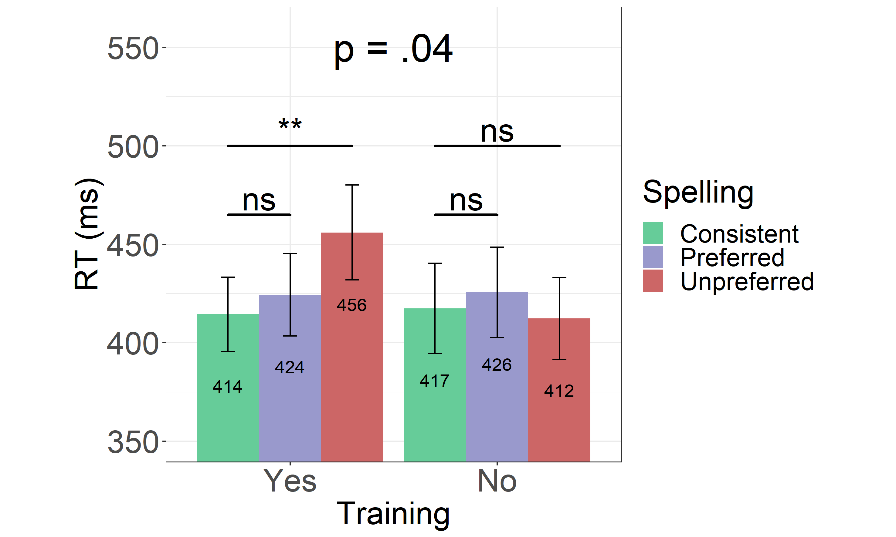
Figure 1.5: Reaction Times From the Experiment 1. Reaction times for for both trained (Yes) and untrained (No) consistent, preferred and unpreferred word spellings. Error bars represent the standard error of the mean.
To sum up, while no differences in RTs were found between consistent and either of the two inconsistent spellings (preferred or unpreferred) in the group of untrained words, trained words presented in their unpreferred spellings yielded significantly longer reading times as compared to the words with consistent spellings.
1.3.2.1 The role of bigram frequencies
To explore the role of bigram frequencies in generating orthographic skeletons, instead of considering participants’ individual preferences, inconsistent words were split in two groups (i.e., classified as preferred or unpreferred) based on bigram frequencies of the target syllables. Bigram frequencies were calculated using B-Pal (Davis & Perea, 2005), and words with initial syllables <ba>, <bu>, <je>, <gi>, <lle>, <llu>, <que> and <qui> were classified as preferred, since they are more frequently present in the initial position of real Spanish words. Their counterparts (i.e., less frequent initial bigrams) were hence considered as unpreferred.5
The full fixed-effects and random-effects structure of the model looking into bigram frequencies is shown in Table 1.6. The model showed neither the interaction between Training and Spelling1vs2 contrast (β = -.018, SE = .035, t = -.524, p = .600) nor the interaction between Training and Spelling1vs3 (β = -.043, SE = .034, t = -1.26, p = .206).
Therefore, the pattern of results observed when considering participants’ personal preferences was not replicated when preferred and unpreferred spellings were inferred from statistical properties of the language (i.e., the bigram frequency).
| Fixed effects | Estimate | SE | t value | p |
|---|---|---|---|---|
| (Intercept) | 5.94 | 0.048 | 124 | < .001*** |
| Training | -0.039 | 0.017 | -2.31 | < .05* |
| Spelling1vs2 | 0.031 | 0.021 | 1.50 | 0.140 |
| Spelling1vs3 | 0.034 | 0.017 | 1.96 | 0.054 |
| Set | -0.139 | 0.096 | -1.44 | 0.154 |
| Training: Spelling1vs2 | -0.018 | 0.035 | -0.524 | 0.600 |
| Training: Spelling1vs3 | -0.043 | 0.034 | -1.26 | 0.201 |
| Random effects | Variance | Std. Dev. | ||
| Participant (Intercept) | 0.108 | 0.329 | ||
| Participant: Training (slope) | 0.004 | 0.066 | ||
| Participant: Spelling1vs2 (slope) | 0.007 | 0.081 | ||
| Participant: Spelling1vs3 (slope) | 0.001 | 0.024 |
1.3.3 Exploratory analysis
As an exploratory question we were interested in the potential relationship between generating orthographic skeletons and retaining the newly acquired words. A measure of participants’ tendency to generated orthographic skeletons was operationalised as a difference in reading previously acquired words shown in their unpreferred and those with consistent spellings (i.e., mean RT) and denoted as the orthographic skeleton effect (OSE). Each participant’s OSE score was then correlated with their performance on the picture naming task (i.e., their inverse ALINE score). Correlations were run for the three different spelling groups separately (see Figure 1.6).
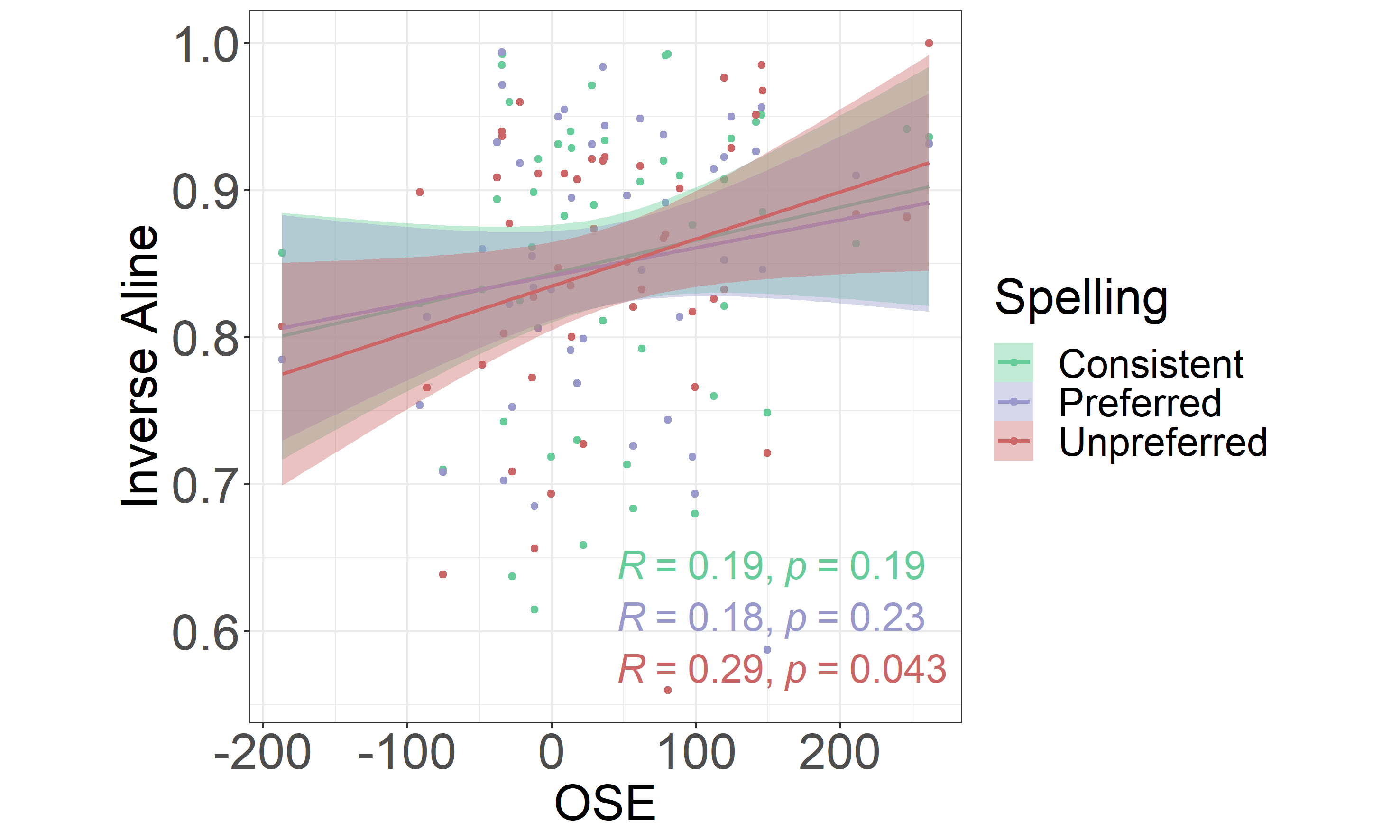
Figure 1.6: Correlation Between the OSE and Word Recall. The OSE (on the x-axis) operationalized as a difference in mean reaction times between the unpreferred and consistent spellings. The higher the value, the larger the effect. Analogously, higher inverse ALINE distance (y-axis) represents higher accuracy in recalling the names of the objects participants were trained on.
As shown in the Figure 1.6, the only significant correlation was the one found between the OSE and the inverse ALINE score for words from the unpreferred spelling group (r(46) = .29, p = .043). This correlation indicates that participants who were more susceptible to generate orthographic skeletons as a result of aural training, were the ones who remembered better the novel words presented in unpreferred spellings in the reading task.
1.4 Discussion
The first experiment of the present thesis aimed to further explore the orthographic skeleton hypothesis by testing whether preliminary orthographic representations are generated for all newly acquired spoken words, or only for words with a unique and hence entirely predictable spellings. To that end, 48 adult speakers of Spanish participated in a two-session online experiment. During Session 1, participants’ individual spelling preferences were collected for all novel words (i.e., both trained and untrained) through a pre-test spelling task. Two weeks later, during Session 2, participants were trained on the pronunciations of novel words that varied in terms of the number of possible spellings: consistent words had only one, while inconsistent words had two possible spellings. Following the aural training, participants were presented with spellings of both trained and untrained words in a self-paced sentence reading task. Significantly longer reading times were observed only for newly acquired words presented in their unpreferred spellings, thereby suggesting that Spanish adult readers had generated orthographic expectations as a result of phonological training. Importantly, they did so for both consistent and inconsistent words (i.e., when there was certainty regarding spelling, but also when there was uncertainty due to inconsistent phonemes). Furthermore, orthographic skeletons for inconsistent items were in line with participants’ individual spelling preferences, given that inconsistent words shown in their preferred spellings did not differ in reading times from words with a single possible spelling (i.e., consistent words). As no significant differences were observed between consistent and inconsistent untrained words, this way yielding a significant interaction between spelling and training, we interpret these findings as evidence that participants indeed generated orthographic skeletons during aural training.
The present study introduces two important innovations: firstly, the number of possible spelling options for each novel word was controlled for by creating words with only one, or two possible spellings. Secondly, participants’ personal spelling preferences were used to determine the preferred spelling option for words with two possible spellings. As a result, we were able to overcome a caveat present in the study conducted by Wegener et al (Wegener et al., 2018) related to the stimuli they used. Since due to high complexity of phoneme-to-grapheme mappings present in the English language, items with predictable and unpredictable spellings could not be matched on number of graphemes, as well as bigram frequency, observed differences between these two groups of items could be at least partly linked to stimuli properties rather than orthographic skeletons participants generated during the learning phase.
Additionally, by assessing individual spelling preferences, and this way determining the orthographic skeleton participants were more likely to generate when two options were available, the present study was also able to address an issue raised by Johnston et al., (2004) concerning individual variability in orthographic expectations. Indeed, in the present study preferred spellings varied considerably across participants (see Appendix 3.6). Interestingly, in some cases, preferred spellings deviated from the orthotactic rules of the language. For example, based exclusively on the frequency of its appearance in Spanish, the grapheme <ll> should be preferred for items with the /ʎ/ sound at the initial position. Looking at Tables in Appendix 3.6, it is clear that this was not the case, since the majority of the participants tested in the study actually preferred the less frequent grapheme <y>. More importantly, as indicated by the absence of an interaction between spelling and training when bigram frequencies, rather than individual spelling preferences, were considered, the latter were indeed favored in generating orthographic skeletons for novel words with two spellings. Nevertheless, although this manipulation allowed us to adapt the stimuli material at the participant level, it introduced a potential confound. Namely, it could be that case that obtaining participants’ spelling preferences beforehand may have influenced their performance on tasks completed two weeks later. To minimize the impact of the pre-test spelling several precautions had been taken: additional filler tasks and filler items were added, and a two-week delay between the sessions was introduced. These precautions seem to have been enough to mask any potential influence of the pre-test task, given that significant differences in reading times were present only for previously trained items, despite the fact that both trained and untrained items have been presented in Session 1. In conclusion, future studies dealing with novel word spellings could, in addition to considering other important psycholinguistic variables, also adapt their material at the participant level.
Further evidence for the orthographic skeleton account comes from the exploratory analysis in which participants’ tendency to generate orthographic skeletons (i.e., the OSE score calculated as a difference in reading times for unpreferred and unique spellings) was correlated with their performance on the picture naming task at the end of the experiment. The significant positive correlation observed only between the OSE score and the accuracy in remembering words shown in their unpreferred spellings, suggests that participants who are more prone to generating orthographic skeletons are also more likely to correctly recall the items encountered in the unexpected spelling, that is, those that deviated from their expectations. The observed relationship between word recall and the surprisal effect in reading (i.e., longer reading times for unpreferred spellings), should however be explored in more detail in order to draw any strong conclusion about its nature. For instance, participants’ tendency to generate orthographic skeletons should be investigated in relation to other constructs shown to play a role in word learning (e.g., phonological short-term memory).
1.4.1 Comparison with Wegener et al. (2018; 2020)
The findings from the present study add to the previous literature by showing that the mechanism driving phoneme-to-grapheme conversions functions even under uncertainty. They therefore expand on the findings reported by Wegener and colleagues (2018, 2020). Nevertheless, this and the two studies by Wegener and colleagues differ in their methodological approaches, leading to differences in the observed results. Firstly, the interaction between spelling and training observed in the present study, was driven by longer reading times present only for previously acquired inconsistent words shown in their unpreferred spellings. The interaction observed in the study conducted by Wegener et al. (2018, 2020) however, stemmed from shorter reading times and consequently a significant facilitation observed only for previously trained words shown in their predictable spellings. We propose several explanations for this reversed pattern of results, and in particular, the absence of training advantage in the present study: first, novel word learning paradigm employed by Wegener et al. (2018, 2020), apart from being more extensive and distributed over two experimental sessions, included both aural and semantic training. By contrast, participants in the present study were exposed to relatively short aural training, with only the picture of the object as semantic context. Their orthographic expectations were tested immediately after, in the course of the same experimental session. This short training, as well as the delay between training and testing, might not have been long enough for the effect of aural training to emerge. Secondly, different techniques were employed, and consequently, the evidence for the orthographic skeleton hypothesis is based on different dependent measures. While the conclusions of the present study come from reading latencies measured through a behavioral response (i.e., button press after reading a word), Wegener and colleagues employed an online measure of the reading process (i.e., eye-tracking). In the same vein, the simplicity of the reading task employed in the present study, which consisted of reading short disyllabic words embedded in relatively simple sentences with no semantic context (see Section 1.2.3.3), might have compromised the likelihood of detecting the training facilitation observed in the previous aural training studies (e.g., Álvarez-Cañizo, Suárez-Coalla, & Cuetos, 2019; Michael Johnston et al., 2004; McKague et al., 2001). Moreover, these studies were conducted in languages with highly distinct writing systems. English, which has been used in all previous studies, has a highly inconsistent orthographic system with both phoneme-to-grapheme as well as grapheme-to-phoneme inconsistencies. This means that both reading as well as spelling unfamiliar words in English comes with high uncertainty (Ziegler, Stone, & Jacobs, 1997). As a result, English speakers are frequently confronted with unexpected spellings. Their scarce experience with predictable spellings could have lead to the facilitation effects in reading previously acquired spoken words in line with their expectations. By contrast, Spanish speakers are rarely confronted with irregular spellings, and may hence be more sensitive to situations in which their expectations are not confirmed (as indicated by longer reading times only for unpreferred spellings). Apart from different techniques, different paradigms and designs, differences in the writing systems also partly explain why trained words did not lead to an overall processing advantage in the current study. Finally, we cannot discard the possibility that differences in reading skills could have also lead to differences in reading trained versus untrained words. In the present study adult skilled readers were tested, whereas Wegener and colleagues tested children developing readers. Compared to developing readers who rely heavily on their phonological decoding skills when reading, and thus need more time to sound out unfamiliar words (Share, 1995), skilled readers are due to their extensive experience and automaticity in reading fast even when reading unfamiliar words. Therefore, any differences between trained and untrained words present in skilled readers might haven been too small to be detected in reading times measured via button presses.
1.4.2 Conclusion
Before concluding, one important limitation of the present study, which will be explored in the remainder of the present thesis, should be mentioned. The conclusion that orthographic expectations are generated even when there is uncertainty regarding the possible spelling (i.e., even for inconsistent items) is based on reading novel words with only two possible spellings. However, it is possible that orthographic skeletons are not generated when the number of possible word spellings larger, and consequently the probability of a mismatch between the expectations and the actual spelling is higher. Moreover, the process of generating orthographic skeletons might also be constrained by the complexity of the specific orthographic system. In languages like Spanish, the overall probability of generating an incorrect orthographic representation is low. As a result, Spanish speakers may be more prone to generating orthographic expectations even when there is uncertainty regarding the correct spelling. Therefore, the ubiquity of skeleton creation when learning novel words with multiple spellings should be explored in other languages with more opaque writing systems. Due to more complex sound-to-spelling rules, opaque languages contain higher level of uncertainty, and consequently higher risk of error when generating orthographic skeletons than Spanish. The generalisability of the results we report here will be investigated in Experiment 2.
References
Note that the lower rate of outlier removal (e.g., removal lower than 1.5 % of the data or even no removal at all) yielded the same pattern of significance in the main analysis.↩︎
Note that this led to an uneven number of items across the two inconsistent groups of items. Namely, given that the items that were for some participants classified as preferred, for the others, those same items were classified as unpreferred. For instance, the item /bumi/, which was originally a preferred item, had to be presented to some participants as <bumi> and to some as <vumi> in the reading task (based on individual spelling preferences). By contrast, following only the bigram frequency, this item was classified as preferred for all participants who saw it with the letter <b> in the task, and as unpreferred for those who saw it with <v>.↩︎